Introduction

In this article, we’ll dive into the world of deep learning with PyTorch by constructing a multiple linear regression model to predict a vehicle’s miles per gallon (MPG) based on various features. We’ll explore the preprocessing steps, model architecture, training process, and evaluation of the model’s performance.

Preparing the Data and Data Preprocessing

Our journey begins by loading the auto MPG dataset, which contains information about vehicle characteristics and their corresponding MPG values. We’ll focus on features like the number of cylinders, displacement, horsepower, weight, acceleration, manufacturing origin, and model year.

To ensure our data is suitable for training, we perform necessary preprocessing steps. We drop rows with missing values, standardize continuous features, and transform categorical features into one-hot encoded vectors.

import pandas as pd
import matplotlib.pyplot as plt

import sklearn
import sklearn.model_selection
import torch
import torch.nn as nn
from torch.nn.functional import one_hot
from torch.utils.data import DataLoader,Dataset,TensorDataset
# Load the dataset
url = 'http://archive.ics.uci.edu/ml/machine-learning-databases/auto-mpg/auto-mpg.data'
column_names = ['MPG', 'Cylinders', 'Displacement', 'Horsepower', 'Weight', 'Acceleration', 'Model Year', 'Origin']

df = pd.read_csv(url, names=column_names,
                 na_values = "?", comment='\t',
                 sep=" ", skipinitialspace=True)


# Dropping rows with missing values

df = df.dropna().reset_index(drop=True)

# Splitting the data into train and test sets
df_train, df_test = sklearn.model_selection.train_test_split(df, train_size=0.8, random_state=1)

# Standardizing continuous features
numeric_column_names = ['Cylinders', 'Displacement', 'Horsepower', 'Weight', 'Acceleration']
train_stats = df_train.describe().transpose()

df_train_norm, df_test_norm = df_train.copy(), df_test.copy()
for col_name in numeric_column_names:
    mean = train_stats.loc[col_name, 'mean']
    std  = train_stats.loc[col_name, 'std']
    df_train_norm[col_name] = (df_train_norm[col_name] - mean) / std
    df_test_norm[col_name] = (df_test_norm[col_name] - mean) / std

# Bucketing the model year categories
boundaries = torch.tensor([73, 76, 79])
 
v = torch.tensor(df_train_norm['Model Year'].values)
df_train_norm['Model Year Bucketed'] = torch.bucketize(v, boundaries, right=True)

v = torch.tensor(df_test_norm['Model Year'].values)
df_test_norm['Model Year Bucketed'] = torch.bucketize(v, boundaries, right=True)

numeric_column_names.append('Model Year Bucketed')

# One-hot encoding the origin feature

total_origin = len(set(df_train_norm['Origin']))

origin_encoded = one_hot(torch.from_numpy(df_train_norm['Origin'].values) % total_origin)

# Creating the train and test feature and label tensors

x_train_numeric = torch.tensor(df_train_norm[numeric_column_names].values)
x_train = torch.cat([x_train_numeric, origin_encoded], 1).float()
 
origin_encoded = one_hot(torch.from_numpy(df_test_norm['Origin'].values) % total_origin)
x_test_numeric = torch.tensor(df_test_norm[numeric_column_names].values)
x_test = torch.cat([x_test_numeric, origin_encoded], 1).float()


y_train = torch.tensor(df_train_norm['MPG'].values).float()
y_test = torch.tensor(df_test_norm['MPG'].values).float()

# Creating a data loader to load the train dataset in batches
train_ds = TensorDataset(x_train, y_train)
batch_size = 8
torch.manual_seed(1)
train_dl = DataLoader(train_ds, batch_size, shuffle=True)

Building the DNN Regression Model

With our data prepared, we move on to constructing our Deep Neural Network (DNN) regression model using PyTorch. This model will predict MPG values based on the vehicle’s features.

# Define the model architecture
hidden_units = [8, 4]
input_size = x_train.shape[1]

all_layers = []
for hidden_unit in hidden_units:
    layer = nn.Linear(input_size, hidden_unit)
    all_layers.append(layer)
    all_layers.append(nn.ReLU())
    input_size = hidden_unit

all_layers.append(nn.Linear(hidden_units[-1], 1))
model = nn.Sequential(*all_layers)

# Define the loss function and optimizer
loss_fn = nn.MSELoss()
optimizer = torch.optim.SGD(model.parameters(), lr=0.001)

Training the Model

It’s time to train our DNN regression model on the training data. We iterate through the data for a specified number of epochs, adjusting the model’s weights to minimize the mean squared error loss.

num_epochs = 200
log_epochs = 20 

for epoch in range(num_epochs):
    loss_hist_train = 0
    for x_batch, y_batch in train_dl:
        pred = model(x_batch)[:, 0]
        loss = loss_fn(pred, y_batch)
        loss.backward()
        optimizer.step()
        optimizer.zero_grad()
        loss_hist_train += loss.item()
    if epoch % log_epochs == 0:
        print(f'Epoch {epoch}  Loss {loss_hist_train/len(train_dl):.4f}')

Epoch 0  Loss 530.7308
Epoch 20  Loss 7.8103
Epoch 40  Loss 7.7546
Epoch 60  Loss 6.9081
Epoch 80  Loss 6.8482
Epoch 100  Loss 6.7144
Epoch 120  Loss 6.4509
Epoch 140  Loss 7.1134
Epoch 160  Loss 6.4428
Epoch 180  Loss 6.2078

Evaluating the Model

Once the model is trained, we assess its performance on the test dataset. This helps us understand how well the model generalizes to new, unseen data.

with torch.no_grad():
    pred = model(x_test.float())[:, 0]
    loss = loss_fn(pred, y_test)
    mae = nn.L1Loss()(pred, y_test)
    print(f'Test MSE: {loss.item():.4f}')
    print(f'Test MAE: {mae.item():.4f}')

Test MSE: 13.1923
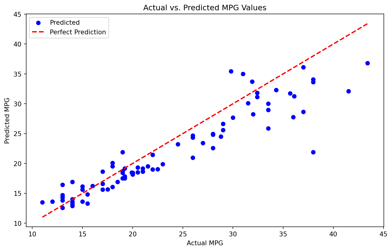
Test MAE: 2.6507

Seeing the good metrics, let’s confirm by plotting the actual and predicted values

# Plotting actual vs. predicted MPG values
plt.figure(figsize=(10, 6))
plt.scatter(y_test, pred, color='blue', label='Predicted')
plt.plot([y_test.min(), y_test.max()], [y_test.min(), y_test.max()], color='red', linewidth=2, linestyle='--', label='Perfect Prediction')
plt.xlabel('Actual MPG')
plt.ylabel('Predicted MPG')
plt.title('Actual vs. Predicted MPG Values')
plt.legend()
plt.show()

Conclusion

Our DNN regression model demonstrates promising results in predicting MPG values based on vehicle features. By carefully preprocessing the data, constructing an appropriate model architecture, and iteratively training the model, we achieve a model that generalizes reasonably well to new data. This article serves as a starting point for your journey into deep learning with PyTorch, enabling you to build more advanced models and tackle a variety of data analysis challenges.